Page 5 of 13
CM6.{3,5-6} | CM6.{3,5-6} | Statistical Analysis and Software Use — SDL Guide
Learning Objectives
- Describe and apply elementary tests of significance — z-test, t-test (one-sample, two-sample, paired), ANOVA, chi-square — in appropriate community medicine study designs (CM6.3)
- Distinguish parametric from non-parametric tests and select the correct test for a given dataset (CM6.3)
- Correctly interpret p-values and 95% confidence intervals, and distinguish statistical from clinical significance (CM6.3, CM6.6)
- Understand the use of statistical software (Epi Info, OpenEpi, SPSS, Excel) for data analysis in community medicine (CM6.5)
- Perform descriptive statistics on a given dataset and interpret the findings in a community medicine context (CM6.6)
INSTRUCTIONS
The previous module gave you the tools to describe data: how to classify, collect, organise, and summarise it with measures of central tendency and dispersion. This module makes the leap from description to inference — from 'what do these numbers show?' to 'can I conclude this is a real difference, or is it just chance?' That leap requires statistical tests of significance, and the choice of the right test is one of the most practically important skills in community medicine research. This module builds that skill through a principled decision framework, worked examples grounded in Indian community medicine contexts, and a practical introduction to the statistical software tools you will use in internship and beyond.
References
- Park K. Park's Textbook of Preventive and Social Medicine, 26th ed. Ch 2 — Epidemiology: Methods (Statistical Tests of Significance) (textbook)
- Indrayan A, Malhotra RK. Medical Biostatistics, 4th ed. Chs 9–12 (Tests of Significance) (textbook)
- Mahajan BK, Gupta MC. Methods in Biostatistics for Medical Students, 8th ed. Chs 5–8 (textbook)
- CDC Epi Info 7 User Guide (https://www.cdc.gov/epiinfo/) (resource)
- OpenEpi — Open-Source Epidemiologic Statistics for Public Health (https://www.openepi.com/) (resource)
Version 2.0 | NMC CBUC 2024
CLINICAL SCENARIO
A district health officer reads a report from the Primary Health Centre: the mean haemoglobin of children under five in villages that received the iron-fortified rice programme is 10.9 g/dL, compared to 10.3 g/dL in villages that did not. The nutritionist declares it a success. But before the State government scales up the programme at a cost of ₹45 crore, the health officer asks a single question: 'Could this 0.6 g/dL difference have occurred simply by chance — even if the programme has no real effect?' That question is answered by a test of statistical significance. Without it, a programme with no real benefit might be scaled up, and a genuinely effective programme might be dismissed as 'only a small difference.' Statistical inference is the tool that separates signal from noise in public health — and this module teaches you to use it.
WHY THIS MATTERS
NMC competency CM6.3 states: 'Describe, discuss and demonstrate the application of elementary statistical methods including test of significance in various study designs.' This is not an abstract mathematical exercise. In community medicine field surveys, cross-sectional studies, and programme evaluations, you will routinely need to determine whether differences between groups are real or due to sampling variation. Tests of significance and confidence intervals appear in every district health survey report, every epidemiological paper, and every programme evaluation you will read or write. CM6.5 (statistical software) and CM6.6 (performing descriptive statistics) are equally practical: Epi Info and OpenEpi are the tools of choice in field epidemiology worldwide, and the ability to enter data, run a test, and correctly interpret the output is a core competency for the National Health Mission health officer you will become.
RECALL
From the previous SDL (Statistical Data Workflow): you can now calculate the mean, SD, and SE of a dataset. Recall that SE = SD/√n and that it measures the precision of the sample mean. You also know that data can be continuous (measured, ratio scale) or categorical (nominal or ordinal). Carry these forward — the choice of statistical test depends entirely on the type of data and the number of groups being compared. Also recall from your Year-1 Physiology discussions: when we say haemoglobin values in a healthy population follow a 'normal distribution,' what does that bell-shaped curve look like, and what percentage of values fall within ±2 SD of the mean? That question will be answered precisely in the next section.
The Burden of Inference Error: Why Statistical Tests Matter in Community Medicine
Every public-health decision involves a choice made under uncertainty. A district programme officer allocates ₹5 crore to a deworming intervention after seeing that dewormed children gained 1.2 kg more than controls. A health minister suspends a vaccination campaign after three adverse events are reported in 100,000 doses. Both decisions could be right — or catastrophically wrong — depending on whether the observed differences reflect real effects or merely chance variation arising from imperfect sampling.
Statistical inference is the formal discipline that quantifies that chance. Its foundation is the null hypothesis (H₀): the assumption that any observed difference is due to chance alone — that there is no real effect. The alternative hypothesis (H₁) states that a real difference exists. A test of significance calculates the probability of observing data as extreme as, or more extreme than, what you actually observed IF H₀ were true. This probability is the p-value.
Two types of inference error are possible, and both carry real public-health costs:
- Type I error (α — false positive): You reject H₀ when it is actually true. You conclude the programme worked when it did not. Cost: money wasted on an ineffective intervention. By convention, α is set at 0.05 (5%): you accept a 5% chance of being wrong in this direction.
- Type II error (β — false negative): You fail to reject H₀ when it is actually false. You conclude no difference when there really is one. Cost: an effective intervention is not implemented; patients continue to suffer a preventable burden. Statistical power (1 − β) is the probability of correctly detecting a real effect. Adequate power (typically ≥80%) requires sufficient sample size — calculated BEFORE data collection.
Understanding these two errors explains why p < 0.05 is a convention, not a law: it represents a policy decision about how to balance false positives against false negatives in public-health decision-making.
Probability, the Normal Distribution, and Confidence Intervals
Statistical tests are grounded in probability theory, and most parametric tests assume that the data — or at least the sampling distribution of the mean — follow a normal (Gaussian) distribution: a symmetrical, bell-shaped continuous probability curve defined entirely by its mean (μ) and standard deviation (σ). Understanding the normal distribution is not an abstract mathematical exercise — it is the reason you can compute a 95% confidence interval, justify a z-test on large samples, and interpret the p-value from a t-test. Without the normal distribution as a foundation, the algebra of significance testing is a set of unexplained recipes rather than a coherent framework. This section builds that foundation explicitly so that the tests in subsequent sections make mechanistic sense rather than having to be memorised by rote.
The normal distribution appears throughout community medicine because many biological variables — height, weight, blood pressure, haemoglobin, serum cholesterol — are approximately normally distributed in large populations. More importantly, even when the original variable is NOT normally distributed, the distribution of sample means approaches normality as the sample size grows, a property formalised as the Central Limit Theorem. This is why statistical tests designed for normal distributions are so broadly applicable in field epidemiology and community health research.
The normal distribution has three properties every community medicine student must know:
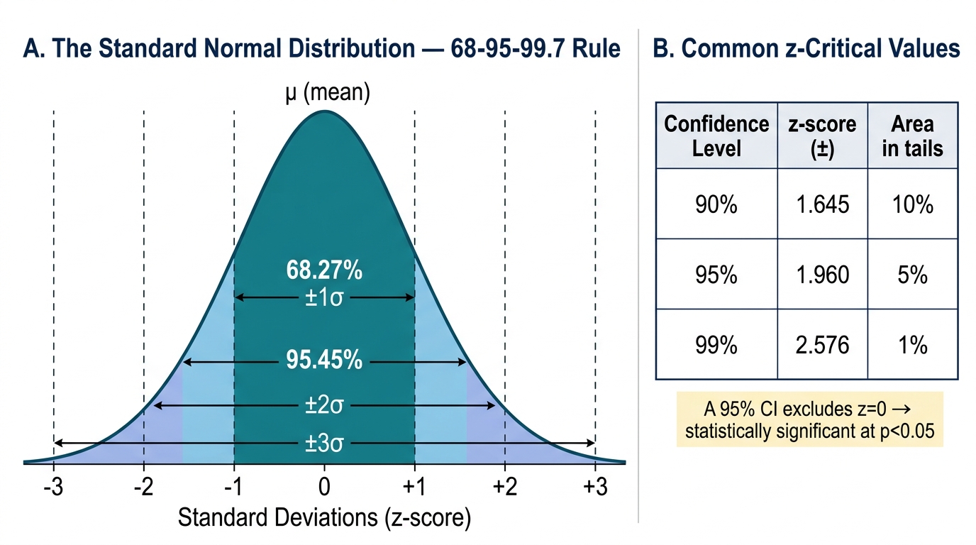
- The 68-95-99.7 rule: approximately 68.27% of values lie within ±1 SD of the mean; 95.45% within ±2 SD; 99.73% within ±3 SD. These are not approximations to memorise by rote — they derive from the mathematical properties of the normal curve and are the basis for constructing confidence intervals.
- The standard normal (z) distribution: any normal distribution can be converted to a standard form with mean = 0 and SD = 1 by computing z = (x − μ) / σ. A z-score tells you how many SDs a value is from the mean. The z-score corresponding to the central 95% of the distribution is ±1.96 — a number you will use in every confidence interval calculation.
- The Central Limit Theorem (CLT): regardless of the shape of the underlying population distribution, the distribution of sample means approaches a normal distribution as sample size increases (n ≥ 30 is the conventional threshold). This is what justifies using z-tests on large samples even when the underlying data are not perfectly normally distributed.
Confidence Intervals (CI) translate the sampling distribution into a directly interpretable range. The 95% confidence interval for a sample mean is:
95% CI = x̄ ± 1.96 × SE
where SE = SD/√n. Interpretation: if the study were repeated many times, 95% of the intervals constructed this way would contain the true population mean. (A common — and important — misconception: the 95% CI does NOT mean 'there is a 95% probability that the true mean lies in this interval.' The true mean either is or is not in any specific interval; probability applies to the procedure, not to a single interval.)
A narrower CI means more precision (achieved by larger n or smaller SD). A CI that does not cross the null value (e.g. 0 for a difference, or 1 for a ratio) indicates statistical significance at the corresponding α level.
The Standard Normal Distribution: 68-95-99.7 Rule and z-Critical Values
SELF-CHECK
A 95% confidence interval for the difference in mean BMI between two groups is 1.2 to 3.8 kg/m². Which statement is correct?
A. There is a 95% probability the true difference is between 1.2 and 3.8 kg/m²
B. The difference is statistically significant at p < 0.05
C. If the study were repeated, the true mean difference would always fall in this interval
D. The difference is not clinically meaningful
Reveal Answer
Answer: B. The difference is statistically significant at p < 0.05
A 95% CI that does not include zero (the null value for a difference) indicates statistical significance at p < 0.05. The CI is 1.2 to 3.8 — it does not cross zero — so the difference is statistically significant. Option A is the most common CI misconception: the 95% refers to the long-run frequency of the procedure, not the probability for a single computed interval. Option C is wrong — the true mean is fixed; it is the interval that varies across repeated studies. Option D cannot be determined from statistical significance alone; clinical significance depends on whether a 1.2–3.8 kg/m² BMI difference is meaningful in the programme context.
Choosing the Right Statistical Test: A Decision Framework
Selecting an inappropriate statistical test is one of the most common methodological errors in medical research — and one of the most tested topics in NMC Theory papers. The decision depends on four factors, applied in sequence: (1) the type of outcome variable (categorical vs continuous), (2) the number of groups being compared (one, two, or three or more), (3) whether groups are independent (different subjects) or paired/matched (same subjects measured twice, or matched pairs), and (4) whether the data meet the assumptions of parametric tests (principally: approximately normal distribution and adequate sample size).
A systematic approach prevents errors. The most consequential decisions are: distinguishing parametric from non-parametric; recognising when paired vs independent tests apply; and knowing when to use chi-square vs Fisher's exact.
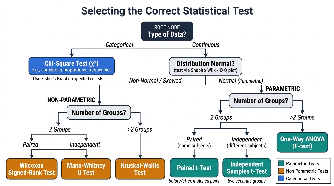
Statistical Test Selection Decision Tree
Parametric tests (require continuous/ratio data, approximately normal distribution):
| Situation | Test |
|---|---|
| Compare sample mean to a known population mean (large n or known σ) | z-test |
| Compare sample mean to population mean (small n, unknown σ) | One-sample t-test |
| Compare means of two independent groups (unknown σ) | Independent two-sample t-test |
| Compare two related measurements (same subjects, before/after or matched pairs) | Paired t-test |
| Compare means of ≥3 independent groups | One-way ANOVA (F-test) |
Non-parametric tests (for ordinal data, non-normal distributions, or small samples):
| Situation | Test |
|---|---|
| Compare two independent groups (ordinal or non-normal continuous) | Mann-Whitney U |
| Compare two related measurements (ordinal or non-normal) | Wilcoxon signed-rank |
| Compare ≥3 independent groups (ordinal or non-normal) | Kruskal-Wallis |
| Association between two categorical variables (expected frequency ≥5) | Chi-square |
| Association between two categorical variables (expected frequency <5) | Fisher's exact |
A high-yield exam point: ANOVA tests for overall significance across ≥3 groups; a significant F does not tell you WHICH pairs differ — post-hoc tests (Tukey's, Bonferroni) are needed for that. For NMC purposes, knowing when to apply ANOVA (rather than multiple t-tests) and the rationale for it (controlling family-wise Type I error) is sufficient.