Page 6 of 13

CM6.{3,5-6} | CM6.{3,5-6} | Statistical Analysis and Software Use — SDL Guide (Part 2)

Parametric Tests: z-test, t-test, and ANOVA

Understanding parametric tests at the conceptual level — what each test assumes, when it applies, and how to interpret its output — is far more valuable than memorising formulas. The three parametric tests you will use most in community medicine practice are the z-test, the t-test (in its three forms), and ANOVA.

z-Test

The z-test compares a sample mean to a population mean when the population standard deviation (σ) is known, OR when the sample size is large (n ≥ 30), using the Central Limit Theorem. The test statistic is:

z = (x̄ − μ₀) / (σ / √n)

For comparing two large-sample means: z = (x̄₁ − x̄₂) / √(s₁²/n₁ + s₂²/n₂). If |z| > 1.96, reject H₀ at α = 0.05. In community medicine, the z-test is commonly used in large epidemiological surveys (e.g. comparing district-level prevalence rates).

t-Tests (Student's t-test)

When population σ is unknown and sample size is small (n < 30), the z-distribution is replaced by the t-distribution, which has heavier tails (more probability in the extremes) to account for the additional uncertainty of estimating σ from the sample. The t-distribution has degrees of freedom (df) that determine its exact shape.

• One-sample t-test: Tests whether a sample mean differs from a known hypothesised value. Example: Is the mean birth weight of babies born at a PHC (sample mean = 2.6 kg, n = 25) significantly different from the national reference of 2.8 kg?

• Independent two-sample t-test: Compares means of two independent groups. Example: Does mean diastolic BP differ between subjects in an exercise intervention group vs a control group (both small samples, σ unknown)? Assumes approximately equal variances (Levene's test checks this).

• Paired t-test: For related measurements — same subject measured twice (pre- and post-intervention) or matched pairs (cases matched to controls on age and sex). The test operates on the differences (d) between pairs: t = d̄ / (SD_d / √n), where d̄ = mean of differences and SD_d = SD of differences. A critical point: paired t-test is NOT a repeated application of the one-sample t-test to each measurement separately — it exploits the correlation between paired observations to reduce variability. Example: haemoglobin before and after 3 months of iron supplementation in 30 women.

ANOVA (Analysis of Variance / F-test)

When three or more independent group means are to be compared, running multiple t-tests inflates the Type I error (three t-tests comparing groups A, B, C give three comparisons, each at α = 0.05, so the family-wise error rate rises above 5%). ANOVA tests whether at least one group mean differs significantly from the others using a single F-statistic:

F = variance between groups / variance within groups

A significant F (p < 0.05) tells you that NOT all group means are equal — but not which groups differ. Post-hoc tests identify the differing pairs. Example: comparing mean haemoglobin across three socioeconomic status groups (low/middle/high) in a cross-sectional survey.

Non-Parametric Tests: Chi-Square, Mann-Whitney, and Kruskal-Wallis

When data are categorical (nominal or ordinal), or when continuous data violate normality assumptions with small samples, non-parametric tests are required. These tests make fewer assumptions about the underlying distribution — they typically operate on ranks or counts rather than raw values — but they are generally less statistically powerful than their parametric equivalents when parametric assumptions ARE met.

Provided image

Chi-Square (χ²) Test

The chi-square test is the workhorse for categorical data in community medicine. It tests whether there is a statistically significant association between two categorical variables in a contingency table. The test statistic is:

χ² = Σ [(O − E)² / E]

where O = observed frequency and E = expected frequency for each cell. Expected frequency for a cell = (row total × column total) / grand total. Degrees of freedom = (rows − 1)(columns − 1).

Key conditions for validity: Expected frequency in EVERY cell must be ≥5. If any expected frequency is <5 (small sample), use Fisher's exact test instead.

Worked example (2×2 contingency table):
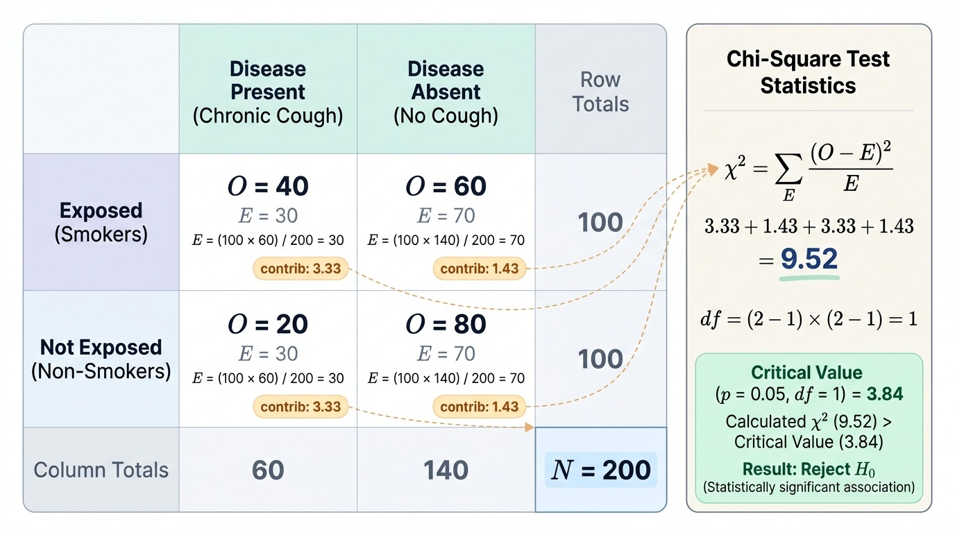
A community health worker surveys 200 adults: 100 are smokers, 100 are non-smokers. Among smokers, 40 have chronic cough; among non-smokers, 20 have chronic cough. H₀: smoking and chronic cough are not associated.

Contingency table:
- Smokers/Cough: O=40, E = (100×60)/200 = 30
- Smokers/No cough: O=60, E=70
- Non-smokers/Cough: O=20, E=30
- Non-smokers/No cough: O=80, E=70

χ² = (40-30)²/30 + (60-70)²/70 + (20-30)²/30 + (80-70)²/70 = 100/30 + 100/70 + 100/30 + 100/70 = 3.33 + 1.43 + 3.33 + 1.43 = 9.52

df = (2-1)(2-1) = 1. Critical value at p < 0.05 with 1 df = 3.84. Since 9.52 > 3.84, reject H₀. Conclusion: there is a statistically significant association between smoking and chronic cough (p < 0.05).

Chi-square for goodness of fit tests whether an observed frequency distribution matches an expected (theoretical) distribution. Example: does the observed blood group distribution in a district match the expected national distribution?

Mann-Whitney U Test

The non-parametric equivalent of the independent two-sample t-test. Used when data are ordinal, or when continuous data are non-normally distributed in small samples. It ranks all observations from both groups combined and compares the rank sums. Example: comparing severity scores (mild/moderate/severe = ordinal) between two treatment groups.

Kruskal-Wallis Test

The non-parametric equivalent of one-way ANOVA. Tests whether ≥3 independent groups come from populations with the same distribution, using rank sums. Example: comparing patient satisfaction scores (ordinal Likert scale) across three different PHC facilities.

Wilcoxon Signed-Rank Test

The non-parametric equivalent of the paired t-test. Used when paired differences are not normally distributed. Ranks the absolute differences and considers their signs. Example: comparing pre- and post-training knowledge scores in a small group of health workers where the differences are not normally distributed.

Interpreting Results: p-values, Confidence Intervals, and Statistical vs Clinical Significance

Obtaining a p-value and a confidence interval is not the end of analysis — it is the beginning of interpretation. Misinterpretation of statistical results is pervasive even in published literature, and the ability to read a results section critically is a core skill for any evidence-based community medicine practitioner. Two kinds of error dominate published misinterpretation: conflating statistical with clinical significance, and treating p-values as statements about the probability of hypotheses rather than about the probability of data. Both errors lead to wrong public-health decisions — scaling up ineffective programmes, or dismissing genuinely beneficial ones. This section gives you the conceptual vocabulary to avoid both traps when reading district health reports, evaluating programme data, or writing your own research conclusions.

To understand what a p-value actually means, it helps to fix the correct interpretation in contrast to the most common wrong ones. The p-value is a statement about the OBSERVED DATA, computed UNDER AN ASSUMPTION about the null hypothesis — it is not a statement about the hypothesis itself. This distinction, while seemingly technical, has profound practical consequences for how you present and interpret community medicine research findings.

The p-value: what it is and what it is not

The p-value is the probability of observing a result as extreme as, or more extreme than, the one obtained, ASSUMING the null hypothesis is true. It is NOT:
- The probability that H₀ is true (a common but incorrect statement)
- The probability that the result occurred by chance
- A measure of the effect size or clinical importance
- A binary verdict (results are not simply 'significant' or 'not significant' — p = 0.049 and p = 0.051 are practically indistinguishable)

A p-value < 0.05 means: IF H₀ were true, there is less than a 5% chance of observing data this extreme. It does not mean the finding is important, large, or clinically meaningful.

Statistical vs clinical significance — the critical distinction

With large sample sizes, trivially small differences become statistically significant. A well-powered study of 100,000 subjects might find a statistically significant mean difference of 0.05 g/dL in haemoglobin between two groups (p < 0.001) — but 0.05 g/dL is below the measurement precision of most haematology analysers and has no clinical meaning whatsoever. Conversely, a small study may fail to detect a clinically important difference due to inadequate power (β error).

Always ask two separate questions: (1) Is the difference statistically significant? (2) Is the effect size clinically meaningful? For community medicine programme decisions, the minimum clinically important difference (MCID) and number needed to treat (NNT) are practical tools for judging clinical significance.

Reporting standards: modern biomedical reporting (CONSORT, STROBE) requires:
- Report the exact p-value (not just p < 0.05 or p = NS)
- Report the effect size with 95% CI
- Include confidence intervals even when p > 0.05 (a non-significant result with a wide CI reflects imprecision, not proof of no effect)

Multiple comparisons problem: when multiple tests are performed on the same dataset, the chance of at least one false positive increases. With 20 independent tests at α = 0.05, one false positive is expected even under H₀. Correction methods include Bonferroni (divide α by number of comparisons) and the False Discovery Rate.